Census Data released yesterday showed that the U.S. rate of homeownership fell from 64.8% in the fourth quarter of 2018 to 64.2% in first quarter of 2019. This was a larger than anticipated drop that put an end to the steady gains that have been made since Q1 2017.

Of the four regions in the U.S., only the South saw homeownership gains, rising from 66% to 66.2%. The Northeast fell from 61.3% to 60.7% and the Midwest fell from 69.3% to 68.2%. The largest decline came in the West where homeownership fell from 60.9% to 59.8%, a drop of more than 1%.

When analyzed by age, the largest drop-off came from those under 35 years of age with the rate falling from 36.5% in Q4 2018 to 35.4 % in Q1 2019. The next largest drop off was for those aged 35 to 44 years, falling from 61.1% to 60.3%. These younger buyers, who had been driving the rise in home ownership over the last couple of years, are now finding it more difficult to find affordable housing. With the average price of housing rising at a faster rate than the average wage increases over the last several years, coupled with a shortage in the supply in start-up housing that has shifted the supply/demand equation, younger buyers are finding it harder to purchase.

Recently, however, home price growth has slowed and interest rates have fallen from 5% down to 4%. Millennials are entering into their early to mid-thirties and still view homeownership as a way of accumulating wealth. These trends have yet to appear in the numbers. As a result, many analysts feel that is quarters downward blip in the numbers might just be an aberration.

When broken out by nationality, Hispanics were the only group to see home ownership gains, rising from 46.9% to 47.4%. By income, those with income less than the median family income saw rates fall from 50.7% to 50.5% while those above the median saw homeowneship fall from 78.9% to 78%.

According to recent report issued by Corelogic, home flipping continues to rise and is currently at the hightes level since they started tracking in 2002. This time however it isn’t just a matter of investors focusing on quick fix based on speculative house price movements, like in the past. Now short-term investors are focused on adding more value to the homes.

In the report the author, Ralph McLaughlin, detailed the following analysis:

"Home Flipping Rates Up Nationally, Highest in Sand States

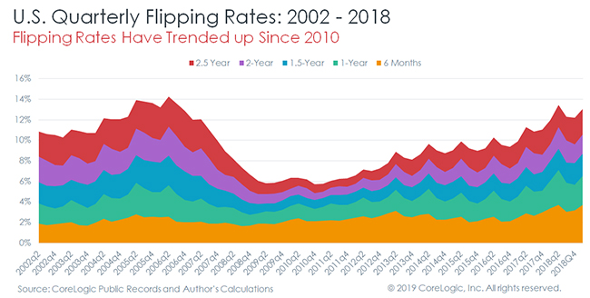
By the fourth quarter of 2018, the flipping rate in the U.S. reached 10.9 percent of all home sales – the fourth highest rate since we started keeping track in 2002, just behind the first quarter of 2018 (11.4 percent, the highest on record), the first quarter of 2006 (11.3 percent), and the first quarter of 2005 (11.1 percent). The flipping rate in the fourth quarter of 2018 was also the highest rate for any fourth quarter in our flipping data series.

While we use the two-year definition of flipping in the remainder of this report, it’s important to also look at how other measures of home flipping have trended over time. As we can see from Figure 1, the fluctuations in flipping activity over time has predominantly occurred not from the involvement of short-term flippers (buying and reselling within 6 months), but rather from longer-term flippers (one year or more). This could be for a few reasons that we’ll investigate in a future report, but it could be a combination of: (1) as prices rise during a housing market expansion, flippers undertake more complicated and time-consuming flips (2) less experienced flippers enter the game, and can’t turn around flips as fast as more experienced flippers, or (3) tax-incentives encourage flippers to take advantage of market appreciation by holding onto properties longer.

Using the two-year definition, we also find that flipping rates vary sharply across the country, tending to be highest in sunbelt metros and lowest in rustbelt metros, although the dichotomy doesn’t fit perfectly. For example, eight of the top ten metros with the highest flipping rate in the fourth quarter of 2018 were in the Sunbelt, with Birmingham, Memphis, and Tampa leading the pack with rates of 16.5, 16.2, and 15.1 percent, respectively. Just two of the top ten were in the rustbelt, with Camden and Philadelphia having rates of 14.9 and 14 percent.

At the low-end, flipping activity tends to be lowest in Rustbelt metros, although two Sunbelt metros, Austin and Houston, make the list with flipping rates at 4.3 and 5.9 percent, respectively. Several metros in Connecticut also lag the country, with Bridgeport, Hartford, and New Haven showing flipping rates of 4.4, 5.1, and 5.3 percent. Five other Rustbelt metros make the list: Springfield, MA, Pittsburgh, PA, Kansas City, MO, Elgin, IL, and Kenosha, WI.

Returns Have Been on a Wild Flipping Ride

In addition to flipping rates, we also estimate economic returns to flipping. What’s the difference between an economic and normal (nominal) returns? Nominal returns are simply the percent difference between what an investor paid a property and what they sold it for, and economic return is the return that excludes opportunity costs, which in the case of flipping is general home value fluctuation. By using economic returns, we can get an idea about whether flippers are adding value of whether they are speculation on market appreciation. See our endnotes for a clarifying example.[iii]

Nationally, we find that gross economic returns in the U.S. have been on a wild ride over our study period. From 2002 – 2007, both economic returns and annualized economic returns (the latter of which controls for the length of a flip) hovered around 4-5 percent. Because closing costs when selling a home are anywhere from 5-8 percent, these findings suggest that the only other way that flippers were trying to make money was by speculating on home value appreciation (remember, economic profits exclude home price appreciation).

After 2007, returns skyrocketed for flippers to a median of around 40 percent (and near 100 percent when annualized), presumably because they were able to purchase distressed properties at deep discounts and quickly resell them at a profit. The fact that annualized returns diverge significantly from non-annualized returns suggests that flippers were quickly reselling their acquired properties, and indeed we find that the median days of flipped home decreased sharply from over 300 days in the mid-2000s to just under 200 days during the foreclosure crisis. Since then, the median time of a flip has rebounded slightly to around 220 days. This shift during the recession caused the annualized returns on home flipping to spike.

As mentioned above, we also find evidence that flippers are shifting away from price speculation and toward adding value to properties. How do we know this? By combining CoreLogic’s public records data with our robust statistical models, we can estimate the discount that a flipper received on a property when they purchased it, and the premium they received when they sold it, relative to similar properties that weren’t flipped. These two metrics, along with market appreciation, are the three ways that flippers can make money on a home.

Just like we found that flippers were likely relying on price speculation from 2002 – 2007, we also find that they weren’t particularly good at buying properties at a discount or selling them at a premium relative to other non-flipped but sold properties during the same time period. Since then, we’ve seen growing signs that flippers are getting increasingly good at buying properties at a discount while the premium they’re selling for has remained mostly constant. This is yet more evidence that flipping today is less risky and less speculative than during the 2000s.

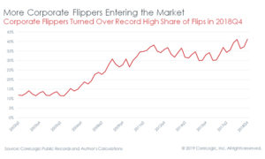
What’s more, the trend away from speculation and toward value-add might be due to an entrance of more experienced, professional flippers into the market. To explore this trend, we looked at the share of flipped homes that were sold by a business entity, such as an LLC, INC, or CORP, rather than by an individual. The trend has clearly been upward, with the share of flipped homes rising to a series high of 41.2 percent in the third quarter of 2018 from a series low of 11.4 percent in the third quarter of 2005.

Returns Highest in Areas with Older Housing

Like flipping rates, we also see substantial variation in economic returns to flipping across U.S. housing markets, with returns highest in the Rustbelt and lowest in the Sunbelt. At the high end, returns are highest in Detroit, Philadelphia, and Pittsburgh with returns of 95.9, 92.8, and 75 percent, respectively. The other seven markets with the highest economic returns to flipping are in Ohio, Maryland, Delaware, Wisconsin, and New York with returns ranging between 58.9 and 70 percent, respectively.

On the low end, flipping returns tend to be lowest in area that have newer housing stock. For example, the three markets with the lowest returns are Raleigh, Colorado Springs, and Charlotte, with returns of 5.1, 7.7, and 7.8 percent, respectively. The other seven markets with the lowest economic returns to flipping are in Arkansas, Missouri, Texas, Arizona, and Tennessee, Florida, and Nevada, with returns ranging between 8.4 and 10.8 percent, respectively.

We can see the relationship between age of homes flipped and economic profits by plotting the median age of home flips against the median economic profits of the 78 markets we have estimates of economic returns. The relationship is quite strong from a statistical perspective, with a R² coefficient of 0.64. This means that 64 percent of the metropolitan-level variation in economic profits can be explained by the variation in the age of homes flipped.

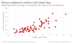
Does this mean that home flippers are reaping more net profits in these older markets? Not so much. While gross economic returns are highest in places with older flips, they don’t capture the amount of money that flippers invested into the flip. On the contrary, flips undertaken on older homes likely require more capital to bring the home up to market standard than newer homes. Such updates might include costly improvements to electrical systems, plumbing, foundations, and roofing. What this does tell us is that flippers are likely to reap substantial discounts when buying properties with such deferred maintenance. In future iterations of our work on flipping, we’ll focus more explicitly on using our vast databases to estimate what improvement were made on a given property, the costs of such work, and thus the net economic profits earned by flippers."

For a more detailed description on the methodologies used in this analysis, please see the full white paper to be presented at the American Real Estate and Urban Economics Association National Conference in May 2019 here.

[i] CoreLogic defines flipping as the purchase of a property with the intent to sell within a two-year period for profit. CoreLogic uses the 24-month definition as that is the Internal Revenue Service’s threshold for when real estate holdings could be considered owner-occupied and thus eligible for capital gains exemptions. The author diverges from previous CoreLogic work on flipping that uses a 12-month definition. This is because 12-month flips only capture flips that are subject to short-term capital gains tax, whereas properties flipped but held for 12-24 months are considered investments but subject to long-term capital gains tax. Since long-term capital gains tax rates tend to be lower than short-term capital gains tax rates, using the 24-month definition thus allows for a much broader analysis of investment in, and returns to, home flipping activity since some flippers may choose to hold properties longer than 12 months so that they may pay the lower long-term capital gains tax rate.

[ii] CoreLogic measures returns as the annualized economic returns to flipping, which considers the opportunity costs of a flip (price growth of similar houses that weren’t part of a flip), any market discount the flipper received on the purchase of the property, and any premium the flipper received on the sale of the property. Because CoreLogic does not observe the capital expenditures that an individual flipper deployed to undertake any renovations or repairs, our estimates of returns represent the upper bound of a return.

[iii] Consider this example: an investor purchases a property for $100,000 and sells it a year later for $200,000 after spending $50,000 on renovations. In this case, they earned a 100 percent gross return and 50 percent net return. However, over the same year, an identical house next door that didn’t have any work done to the property went up in value by $25,000. In this scenario, the gross economic return to the investor would be 75 percent, since we exclude the $25,000 the flipper would have made just from market appreciation. Considering the $50,000 the investor put into the property as well as the $25,000 market appreciation means the flipper earned $25,000, or 25 percent, net economic profit.

In a recently posted article, Edward J. Pinto, a resident fellow and the codirector of the Center on Housing Markets and Finance at the American Enterprise Institute (AEI), took aim at the usefulness of the 30- year mortgage. His feeling is that the slow amortization makes it nearly twice as risky as a similar loan with a 20-year term and that the 30-year compounds risk layering by promoting the use of higher combined loan-to-value (LTV) and debt-to-income (DTI) ratios.

[caption id="attachment_12024" align="alignleft" width="163"] Edward Pinto, Codirector, AEI Center on Housing Markets and Finance; Resident Fellow.[/caption]

Not only is the 30-year loan riskier, according to Mr. Pinto, but the 30-year loan also makes housing less affordable. “The Housing Lobby unabashedly supports the broad availability of the 30-year mortgage, and even wants it extended to manufactured housing. This is because Housing Lobby sees the slow amortization as a feature that reduces monthly payments, making home “more affordable”. They choose to ignore the bug–the 30-year loan, when combined with other risk factors, drives up home prices when the supply of homes is tight, especially for buyers of entry-level homes. Since 2012, lower priced entry-level homes have risen by about 55%, while move-up homes have risen by about 31%. This means lower priced entry-level homes that cost an average of $103,315 in 2012, cost a whopping $160,138 in late-2018. Thus, rather than making housing more affordable as its supporters claim, 30-year loans make housing less affordable. But more on this entry-level home pricing penalty later.”

In his paper he then goes on to outline ten facts to support his case:

“Fact 1: In December 2018, 30-year loans constituted 99% of all government guaranteed loans to finance a home purchase. Government agencies guaranteed 85% of home purchase loans.

Fact 2: This was not always the case. In 1953, the year before Congress authorized the FHA to insure 30-year loans on existing homes, FHA’s average loan term was 21 years and conventional loans had a term of 15 years. Even as recently as 1992, 27% of home purchase loans had a term of 15- or 20-years.

Fact 3: 30-year loans are much riskier than the 15- and 20-year loans they replaced. In general, a 30-year loan is about twice as risky as a 20-year loan with similar risk characteristics. A 15-year loan has about 60% less risk than a 30-year loan with similar characteristics. With the loans terms prevalent in the 1950s, it comes as no surprise that foreclosure levels in the 1950s literally rounded to zero. With the broad adoption of the 30-year loan by FHA in the late 1950s and early 1960s, foreclosure rates started to rise to concerning levels in the early 1960s.

Fact 4: The prominent feature of 30-year loans is its lower or “easier” monthly payment compared to say a 20-year loan. For example, the monthly payment at 4.5% on $100,000 is $507 for a 30-year loan, compared to $633 for a 20-year loan, an increase of 25% per month.

Fact 5: But it is the 30-year loan’s lower monthly payment that is its flaw. The pace of principal pay-down on a 30-year mortgage is agonizingly slow. At the end of 6 years, the balance on the 30-year loan is $89,138, compared to $78,749 for the 20-year loan. This helps explain why the 30-year loan is so much riskier. The paying down of principal through scheduled amortization is called earned equity. House price appreciation through rising prices, particularly when rising faster than inflation, is call unearned equity. Since the long-term success of the 30-year loan as a wealth building tool is reliant on large doses of unearned equity on entry level-homes, it is fatally flawed.

Fact 6: History has shown that the 30-year’s lower monthly payment does not make homes more affordable. Instead, it leads to faster median home price growth relative to median incomes. Back in the 1950s, before the large-scale adoption of the 30-year loan, the median home price was about 2 times median income. Today, this ratio is over 3.5. This result is predictable, as Ernest Fisher, FHA’s first chief economist in the 1930s and a university professor in the 1950s, observed that in a seller’s market, “more liberal credit is likely to be [capitalized] in price.”

Fact 7: As the easy terms of the thirty-year loan gets capitalized into higher home prices, the dollars needed for a down payment of say 10% doubles as the price of a home doubles. Yet as already noted, incomes (and savings) do not rise as quickly. At the start of the current home price boom in 2012, first-time FHA buyers had a median down payment of $3800. In January 2019 the median down payment was still $3800, yet the median home price purchased had increased by 31%. This translates into more risk.

Fact 8: A similar trend has occurred with respect to borrower DTIs. Since 2012, the DTIs of first-time FHA buyers have increased by 13%, an unsurprising result since wages have increased by only about 16% over the same period, but the price of homes purchased went up by 31%.

Fact 9: The impact on the level of risk different borrowers take may be quantified. Loans to first-time buyers that are guaranteed by Federal agencies have an average mortgage risk score of 17%, almost double the rate of 9.9% for repeat buyers.

Fact 10: As noted previously, since 2012 the constant quality price of entry-level homes has risen by about 55%, while move-up homes have risen by about 31%. Had the low segment risen at the same rate as the move-up segment over this period, the average entry-level buyer would be spending $24,800 or 15.5% less for a home today. At this lower price, not only would homes be more affordable but they would require smaller down payments and low DTIs, thereby reducing the risk of foreclosure.”

The result, says Mr., Pinto, is that first time buyers are put in a bad position and are penalized with higher prices. The solution, he suggests, is to use the 20-year loan build wealth more reliably and at a much lower risk of default and adopt policies to increase the supply of newly constructed entry-level homes.